Neural Network Fundamentals
Weights and Bias
Weights (W)
Weights determine how important each input feature is.
A neural network layer computes:
z = w₁x₁ + w₂x₂ + w₃x₃ + ...
Where x₁, x₂, x₃ are inputs and w₁, w₂, w₃ are weights. Each input is multiplied by a weight.
Bias (b)
The bias is an additional value added to the weighted sum.
z = (w₁x₁ + w₂x₂ + ... + wₙxₙ) + b
Bias shifts the output up or down, allowing the model to fit data more flexibly while applying the activation function.
Activation Functions
Introduce non-linearity: they determine whether a neuron should "fire" (activate) based on weighted input, enabling networks to learn complex, non-linear data patterns.
- Sigmoid
- ReLU
- Tanh (Hyperbolic Tangent)
- Leaky ReLU
Softmax
Softmax is usually applied in the last layer of a model.
It converts raw scores (logits) into probabilities.
Properties
- The output values sum to 1
- The token with the highest probability will have a value closer to 1
Sigmoid
The sigmoid function squashes values into a range between 0 and 1.
Commonly used for:
- Binary classification
- Probability outputs
Training Concepts
Loss Functions
A loss function measures how far the model's predictions are from the true values. The goal of training is to minimise the loss.
- Mean Squared Error (MSE) – used for regression; penalises large errors heavily
- Mean Absolute Error (MAE) – used for regression; more robust to outliers than MSE
- Binary Cross-Entropy – used for binary classification; measures difference between predicted probability and true label
- Categorical Cross-Entropy – used for multi-class classification; compares predicted probability distribution to the true class
- Sparse Categorical Cross-Entropy – same as categorical cross-entropy but accepts integer class labels instead of one-hot vectors
Learning Rate
The learning rate is a hyperparameter that controls how much the model's weights are updated during each step of training.
new_weight = old_weight − learning_rate × gradient
- Too high → the model overshoots the optimal weights, training becomes unstable or diverges
- Too low → the model learns very slowly and may get stuck in local minima
- Just right → the model converges efficiently to a good solution
The most common optimiser used to manage the learning rate during training is Adam (Adaptive Moment Estimation), which automatically adjusts the learning rate per parameter based on past gradients.
Vanishing Gradient vs Exploding Gradient
During backpropagation, gradients are multiplied through each layer. Depending on the magnitude of these gradients, two problems can arise:
Vanishing Gradient
Gradients become extremely small as they propagate back through many layers, causing early layers to stop learning.
- Common with sigmoid and tanh activation functions (their derivatives are < 1)
- Especially problematic in deep networks and vanilla RNNs processing long sequences
- Solutions: use ReLU activations, batch normalisation, residual connections (skip connections), or gated architectures like LSTM / GRU
Exploding Gradient
Gradients become extremely large, causing weights to update by huge amounts and making training unstable (loss may spike or become NaN).
- Common in deep networks and RNNs when weight matrices have large values
- Solutions: gradient clipping (cap gradients at a maximum value), proper weight initialisation, batch normalisation
Quick Comparison
                    Vanishing Gradient          Exploding Gradient
Gradients           → 0 (shrink to zero)        → ∞ (grow unbounded)
Effect              Early layers stop learning   Training becomes unstable
Common cause        Sigmoid/Tanh activations     Large weight matrices
Key fix             ReLU, LSTM/GRU, ResNets      Gradient clipping
Model Architectures
Convolutional Neural Networks (CNNs)
CNNs are commonly used for computer vision tasks.
Used For
- Image classification
- Object detection
- Medical imaging
Core Components
- Convolution Layers – extract features from images
- Pooling Layers – reduce spatial size and computation
- Activation Functions – introduce non-linearity
- Fully Connected Layers – produce final predictions
Popular Architectures
- ResNet
- VGG
- EfficientNet
Sequence Models / RNN
Recurrent Neural Networks (RNN)
RNNs have memory, allowing them to process sequential data.
Common Applications
- Machine translation
- Autocomplete
- Sentiment analysis
- Named Entity Recognition (NER)
- Time series prediction
Key Idea
We unroll the data across time steps, while keeping the same weights and biases shared across the sequence.
Key Limitations
- Vanishing / Exploding Gradients – during backpropagation through time (BPTT), gradients are multiplied at each time step; over long sequences they shrink to near-zero (vanishing) or grow unboundedly (exploding), making it hard to learn long-range dependencies
- Short-Term Memory – vanilla RNNs struggle to retain information from early time steps, so context from the beginning of a long sequence is effectively lost by the end
- Sequential (Non-Parallelisable) Processing – each time step depends on the previous hidden state, so RNNs must be processed one step at a time and cannot leverage GPU parallelism the way Transformers can, making them slow to train on long sequences
LSTM and GRU architectures address limitations 1 and 2 with gating mechanisms, but the fundamental bottleneck of sequential processing remained. These limitations directly motivated the landmark 2017 paper "Attention Is All You Need" (Vaswani et al.), which introduced the Transformer architecture — replacing recurrence entirely with self-attention and solving all three limitations.
Gradient and Backpropagation
Reference: https://www.youtube.com/watch?v=LHXXI4-IEns
Seq2Seq Models
A sequence-to-sequence (seq2seq) model maps a variable-length input sequence to a variable-length output sequence. It was the dominant architecture for tasks like machine translation, text summarisation, and dialogue generation before Transformers.
The Original Encoder–Decoder Architecture
The classic seq2seq model (Sutskever et al., 2014) consists of two RNNs (typically LSTMs):
Input: "I love NLP"

Encoder RNN
  "I" → h₁ → "love" → h₂ → "NLP" → h₃  ──► context vector (c)

Decoder RNN
  c → "J'" → "adore" → "le" → "TAL" → <EOS>
- Encoder – reads the entire input sequence token by token and compresses it into a single fixed-size vector called the context vector (the final hidden state)
- Decoder – takes the context vector and generates the output sequence one token at a time, using each previously generated token as input for the next step
The Bottleneck Problem
The entire input sequence is squeezed into one fixed-size context vector. For long sentences this vector cannot retain all the information, causing the model to forget early parts of the input. Translation quality dropped sharply as sentence length increased.
Long input sentence
  ┌──────────────────────────────────────────┐
  │ word₁  word₂  word₃  ...  word₅₀  word₅₁│
  └──────────────────────────────┬───────────┘
                                 ▼
                      Single context vector (c)   ← information bottleneck
                                 ▼
                          Decoder output
The Fix: Attention Mechanism (Bahdanau et al., 2015)
Instead of relying on a single context vector, the attention mechanism lets the decoder look back at all encoder hidden states at every decoding step and decide which parts of the input to focus on.
Encoder hidden states:  h₁   h₂   h₃   h₄   h₅
                         ↑    ↑    ↑    ↑    ↑
                        0.05 0.10 0.60 0.20 0.05   ← attention weights (sum to 1)
                         │    │    │    │    │
                         └────┴────┴────┴────┘
                                  ▼
                         Weighted context vector  → fed into decoder at this step
- Score – at each decoder step, compute an alignment score between the current decoder state and every encoder hidden state
- Normalise – pass the scores through softmax to get attention weights
- Weight – multiply each encoder hidden state by its attention weight and sum them into a new, step-specific context vector
- Decode – feed this context vector (along with the previous token) into the decoder to produce the next output token
Why Attention Solved the Bottleneck
- No more single vector – the decoder gets a fresh, relevant context vector at every step instead of one compressed summary
- Long-range access – the model can attend to any part of the input regardless of sequence length
- Interpretable – attention weights show which input tokens the model focuses on for each output token (useful for debugging translations)
From RNN Attention to Self-Attention (Transformers)
RNN-based attention still had to process the encoder sequentially, one token at a time. The Transformer (Vaswani et al., 2017) replaced the RNN entirely with self-attention, allowing all tokens to attend to each other in parallel — solving the speed bottleneck while keeping the benefits of attention.
Seq2Seq Evolution:

Vanilla Seq2Seq (2014)    Fixed context vector          → bottleneck on long sequences
+ Attention (2015)        Dynamic context per step      → solved information loss
Transformer (2017)        Self-attention, fully parallel → solved speed and scalability
Transformers
Positional Encoding
Positional encoding assigns a numerical representation to each word before embedding, allowing the model to understand the order of tokens in a sequence.
BERT vs GPT
BERT: Autoencoding encoder-only model that reads the entire sequence bidirectionally, excelling at understanding tasks (classification, NER, question answering). Trained with Masked Language Modelling (MLM) — randomly masks tokens in the input and trains the model to predict them using the full surrounding context.
GPT: Autoregressive decoder-only model that processes tokens left-to-right, suited for text generation. Trained with causal language modelling — predicts the next token using only prior context.
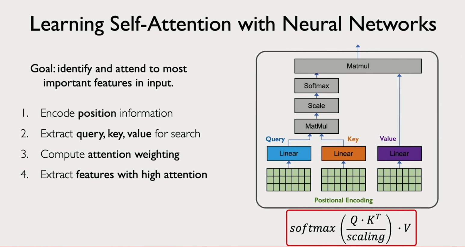
Attention Mechanisms
Attention
Attention allows a model to capture relationships between tokens in a sequence.
This is particularly important in encoder–decoder architectures such as machine translation systems.
Self-Attention
Self-attention allows a model to process an entire sequence simultaneously and learn dependencies between all tokens.
This is powerful for tasks that require understanding context across the whole sequence, such as:
- Text generation
- Question answering
- Summarization
Multi-Head Attention
Multi-head attention runs the attention mechanism multiple times in parallel, each time with different learned weight matrices. Each parallel run is called a head.
Each head can learn to focus on a different type of relationship in the sequence — for example, one head might attend to syntactic structure while another attends to semantic similarity.
The outputs of all heads are concatenated and projected into a final representation.
Input
  |
  +---> Head 1 (Q1, K1, V1) ---> Attention output 1
  +---> Head 2 (Q2, K2, V2) ---> Attention output 2
  +---> Head 3 (Q3, K3, V3) ---> Attention output 3
  |
  +--> Concatenate all outputs --> Linear projection --> Final output
Why it matters: a single attention head can only learn one way to relate tokens. Multiple heads let the model capture several different relationships simultaneously, which is key to the power of Transformers.
Text Representation & Retrieval
Embeddings & Text Representation Techniques
Embeddings are the mathematical representations of words, phrases, or tokens in a large-dimensional space, capturing their semantic meaning and relationships with other words. Before modern embeddings, several simpler techniques were used.
One-Hot Encoding
Each word is represented as a vector of zeros with a single 1 at the word's index in the vocabulary.
Vocabulary: [cat, dog, fish]

cat  →  [1, 0, 0]
dog  →  [0, 1, 0]
fish →  [0, 0, 1]
Problem: no sense of similarity — cat and dog are just as "different" as cat and fish. Vector size grows with vocabulary (sparse, high-dimensional).
N-Grams
Instead of single words, capture sequences of N consecutive words to preserve some context.
Sentence: "I love NLP"

Unigrams (1-gram): [I, love, NLP]
Bigrams  (2-gram): [I love, love NLP]
Trigrams (3-gram): [I love NLP]
Why useful: captures local word order and phrases. "not good" as a bigram is very different from "good" alone.
Problem: vocabulary explodes with larger N, still no semantic meaning.
Bag of Words (BoW)
Represents a document as a vector of word counts, ignoring order entirely.
Vocabulary: [I, love, NLP, AI]

"I love NLP"  →  [1, 1, 1, 0]
"I love AI"   →  [1, 1, 0, 1]
Problem: no word order, no context, all words treated equally.
TF-IDF
Improves BoW by weighting words based on how frequent they are in a document vs. how common they are across all documents. Rare but frequent words in a doc get high scores.
Problem: still no semantic meaning, synonyms treated as unrelated.
Word Embeddings (Word2Vec, GloVe)
Dense low-dimensional vectors where similar words are close in vector space. Captures semantic relationships learned from large corpora.
King − Man + Woman ≈ Queen
Word2Vec Architectures
- CBOW (Continuous Bag of Words) – predicts the target word from surrounding context words. Faster to train and works better for frequent words.
- Skip-gram – predicts surrounding context words from the target word. Works better for rare words and smaller datasets.
Both use a shallow neural network (single hidden layer) and are trained on large text corpora using techniques like negative sampling to make training efficient.
Limitations of Word2Vec
- Static embeddings – one fixed vector per word regardless of context. "bank" (river) and "bank" (money) get the same vector (polysemy problem).
- Out-of-vocabulary (OOV) – cannot handle words not seen during training. Misspellings or new words have no representation.
- No subword information – treats each word as an atomic unit, so it cannot leverage morphology (e.g., "unhappiness" shares nothing with "happy"). FastText addresses this by using character n-grams.
- Requires large corpora – needs substantial training data to produce high-quality embeddings; performs poorly on small or domain-specific datasets.
- No sentence/document-level meaning – only produces word-level embeddings; doesn't capture phrase or sentence semantics directly.
- Encodes societal biases – reflects biases present in the training data (e.g., gender or racial stereotypes in analogy tasks).
Contextual Embeddings (BERT, GPT)
Each word gets a different vector depending on its surrounding context. "bank" in a financial sentence gets a different embedding than "bank" in a nature sentence.
These are the embeddings used in modern Transformers and LLMs.
Evolution Summary
One-Hot Encoding   →  sparse, no similarity
N-Grams            →  adds local context, still sparse
Bag of Words       →  word counts, ignores order
TF-IDF             →  weighted counts, still no semantics
Word2Vec / GloVe   →  dense, semantic, but context-free
BERT / GPT         →  dense, semantic, context-aware
Chunking Methods
Chunking is the process of splitting large documents into smaller pieces before embedding and retrieval.
- Fixed-size Chunking – splits text into chunks of a set character/token length, regardless of content
- Content-aware Chunking – splits at natural boundaries like sentences or paragraphs to preserve meaning
- Recursive Character Level Chunking – recursively splits on a hierarchy of separators (e.g. paragraphs → sentences → words) until chunks are small enough
- Document Structure-based Chunking – uses the document's own structure (headings, sections, markdown) to define chunk boundaries
- Contextual Chunking with LLMs – uses an LLM to intelligently determine the best split points based on semantic context
Hyperparameters
What Are Hyperparameters?
Hyperparameters are configuration values set before training begins. Unlike model parameters (weights and biases), they are not learned from data — you choose them manually or via search.
Training Hyperparameters
Learning Rate
Controls how large each weight update step is. The single most impactful hyperparameter.
Too high  → overshoots optimum, loss diverges
Too low   → learns very slowly, may get stuck
Typical range: 1e-5 to 1e-1  (e.g. 3e-4 for Adam)
Batch Size
Number of training samples processed before the model's weights are updated.
- Larger batch → more stable gradient estimates, faster GPU utilisation, but needs more memory and may generalise worse
- Smaller batch → noisier updates, acts as regularisation, trains more slowly per epoch
- Typical values: 16, 32, 64, 128, 256
Epochs
One epoch = one full pass through the entire training dataset.
- Too few → underfitting
- Too many → overfitting (use early stopping to mitigate)
Optimizer
Algorithm used to update weights. Common choices:
- SGD – simple, often needs careful tuning
- Adam – adaptive learning rate per parameter; most common default
- AdamW – Adam with decoupled weight decay; preferred for Transformers
Weight Decay (L2 Regularisation)
Penalises large weights to reduce overfitting. Added directly to the loss.
loss_total = loss + λ × Σ(w²) where λ is the weight decay coefficient
Dropout Rate
Fraction of neurons randomly set to zero during each training step, forcing the network not to rely on any single neuron.
Typical range: 0.1 – 0.5
0.0 = no dropout (disabled)
0.5 = 50% of neurons dropped each step
Gradient Clipping
Caps gradients at a maximum norm before the weight update, preventing exploding gradients.
Common value: max_norm = 1.0
Architecture Hyperparameters
Number of Layers (Depth)
How many stacked layers the network has. Deeper networks can learn more complex features but are harder to train and prone to vanishing gradients.
Hidden Size / Model Dimension (d_model)
Width of each layer — the size of the internal representation vectors.
GPT-2 small:  d_model = 768
GPT-3:        d_model = 12,288
Number of Attention Heads
In Transformer models, how many parallel self-attention heads to run. Each head attends to different relationships. Must divide evenly into d_model.
head_dim = d_model / num_heads
e.g. 768 / 12 = 64 dimensions per head
Context Length (Sequence Length)
Maximum number of tokens the model can process at once. Attention scales quadratically with sequence length (O(n²)), so longer contexts are expensive.
Feedforward Dimension
Size of the inner layer in the Transformer's feedforward block. Typically 4× d_model.
Inference / Generation Hyperparameters
Temperature
Scales the logits before softmax to control randomness of output.
Temperature = 0.0  → greedy (always picks highest probability token)
Temperature = 1.0  → standard distribution (default)
Temperature > 1.0  → more random / creative
Temperature < 1.0  → more focused / deterministic
Top-k Sampling
At each step, only the k highest-probability tokens are considered. The model samples from these k candidates.
k = 1   → greedy decoding
k = 50  → common default
Top-p (Nucleus) Sampling
Instead of a fixed k, consider the smallest set of tokens whose cumulative probability exceeds p. Adapts dynamically to the distribution shape.
p = 0.9 → sample from tokens covering 90% of the probability mass
Max New Tokens
Hard limit on how many tokens the model generates in one call, preventing runaway outputs.
Repetition Penalty
Reduces the probability of tokens that have already appeared, discouraging repetitive output. Values > 1.0 penalise repetition.
Quick Reference
Hyperparameter          Typical Range / Values       What it controls
────────────────────────────────────────────────────────────────────────
Learning rate           1e-5 – 1e-1                  Step size of weight updates
Batch size              16 – 512                     Samples per update step
Epochs                  1 – 100+                     Full passes through data
Dropout                 0.1 – 0.5                    Regularisation strength
Weight decay (λ)        1e-4 – 1e-1                  Penalty on large weights
Gradient clip           0.5 – 5.0                    Max gradient norm
d_model                 128 – 12,288                 Layer width
Num heads               4 – 96                       Parallel attention heads
Context length          512 – 128,000 tokens         Max input length
Temperature             0.0 – 2.0                    Output randomness
Top-k                   1 – 100                      Candidate token pool
Top-p                   0.5 – 1.0                    Nucleus probability mass
LLM Training & Deployment
LLM Fine-Tuning Methods
- Full Fine-Tuning
- LoRA / PEFT
- Prompt Tuning
FP16 Memory Calculation
FP16 (16-bit floating point) uses 2 bytes per parameter.
Example – 7B parameter model:
7B × 2 bytes = 14 GB
So a 7B parameter model in FP16 requires about 14 GB of RAM.
KV Cache (Key-Value Cache)
During autoregressive generation, a Transformer decoder produces tokens one at a time. At each step, the self-attention mechanism needs the Key and Value vectors of every previous token to compute attention. Without caching, the model would have to recompute K and V for the entire sequence from scratch at every single step.
The Problem Without KV Cache
Generating token 5:
  Must attend to tokens 1, 2, 3, 4
  → recompute K and V for ALL of them

Generating token 6:
  Must attend to tokens 1, 2, 3, 4, 5
  → recompute K and V for ALL of them AGAIN

This is redundant — K and V for tokens 1–4 haven't changed!
How KV Cache Works
The KV cache stores the Key and Value matrices from all previous tokens so they are computed only once and reused at every subsequent step.
Step 1: process token 1 → compute K₁, V₁ → store in cache
Step 2: process token 2 → compute K₂, V₂ → append to cache → attend using [K₁K₂], [V₁V₂]
Step 3: process token 3 → compute K₃, V₃ → append to cache → attend using [K₁K₂K₃], [V₁V₂V₃]
...
Only the NEW token's Q, K, V are computed — past K, V are read from cache
Why It Matters
- Massive speedup — without the cache, generation time scales quadratically with sequence length (O(n²)); with the cache, each new step is O(n) since only one new token's Q attends to all cached K/V
- Trades memory for speed — the cache consumes GPU memory that grows with sequence length, number of layers, and number of attention heads
KV Cache Memory Formula
KV cache size = 2 × num_layers × num_heads × head_dim × seq_len × bytes_per_param

Example — 7B model (32 layers, 32 heads, head_dim=128, FP16, 4096 tokens):
  = 2 × 32 × 32 × 128 × 4096 × 2 bytes
  = ~2 GB
For long context windows (e.g. 128K tokens), the KV cache alone can exceed the model weights in memory.
Optimisations
- Multi-Query Attention (MQA) — all heads share a single set of K, V projections, drastically reducing cache size
- Grouped-Query Attention (GQA) — a middle ground where groups of heads share K, V (used in LLaMA 2 70B, Mistral)
- Quantised KV cache — store cached K, V in lower precision (e.g. INT8) to reduce memory
- Sliding window attention — only cache the most recent N tokens instead of the full history (used in Mistral)
Quick Summary
Without KV cache    Recompute all K, V at every step     Slow (O(n²) per token)
With KV cache       Store and reuse past K, V             Fast (O(n) per token)
Trade-off           Uses extra GPU memory                 Grows with sequence length